I mentioned before about a great tool for AdWord campaigns namely the editor. After the editor, my other favourite programs (I know I’m darn cool) are without doubt Microsoft Excel and Google Analytics. I harp on about GA (Analytics) a lot to both client and colleagues alight but Excel not so much.
Hence this blog.
Excel is great. It is your friend. It’s designed with tasty data in mind, so on that note my next few blogs are doing to be Excel tool based.
First one, pivot tables. Data summary on steroids.
Now, I worked in search for quite a while before I discovered this bad boy. Was at a seminar and we had a lot of keyword data we needed to quickly analyse. Boom, the presenter shoved it into a pivot and off she went. Much to my geeky starry eyed amazement.
So pivot table. Assuming it’s AdWords data, download it – good start. Then, CTRL + 8 to highlight all the data, then to ‘Insert’ far left, ‘Pivot Table’. Click ok on the next box and voila. You should get the below:
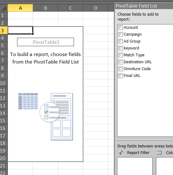
You should also get on the right a ‘Field List’ which allows you to select the data you want to analyse. It also allows you to place it in terms of how you want to view it. i.e do you want to see keyword activity by week, or campaign activity and associated CPC? Whatever is in the table the pivot can calculate. You can either chuck this straight into the table by dragging and dropping or drop it into the fields below.
Top ‘ Report Filter’ indicates what you can drag to the top box for later filtering. This is handy if you know you want to compare WoW or even campaign by campaign. Column indicates the values to the report filter.
Row labels indicates what you want on the left hand side, with values being the associated metrics to your row. I.E throw ‘Campaign’ into the Row column and then add impressions, clicks and ctr to the values and it will bring it up.
Once you have that sorted, open any drop tab next to the text and you should be able to further filter the data.
Best thing is to just have a play around with it. Figure it out.
Something you might notice is CTR summing, no problem. Just right click it, ‘Summarize Values by’ select average and if you need more options for decimal points, it’s at the bottom.
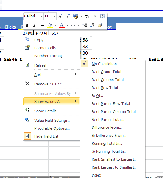
You can also summarise by value, i.e. top ten which is handy for top converting keywords.
Things that are needed are that your data needs to have headers on each columns. No merged cells and it doesn’t always like empty columns.
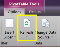
Word to note, if you amend data on the main source data sheet – the tab the pivot is pulling the data from you will need to refresh the pivot. It won’t automatically do this.
But that’s also easy. Just under ‘Options’ it’s the big refresh bar.
You’re welcome. Go forth and pivot that data.